Simple visualisation of a CMIP6 dataset with Python Xarray#
this is an adoption of NordicESMhub example to use CMIP6 data stored in the DKRZ data pool
filename = '/work/ik1017/CMIP6/data/CMIP6/CMIP/NCAR/CESM2/historical/r1i1p1f1/Amon/tas/gn/v20190308/tas_Amon_CESM2_historical_r1i1p1f1_gn_185001-201412.nc'
Import python packages#
import xarray as xr
import cartopy.crs as ccrs
import matplotlib.pyplot as plt
import numpy as np
import cftime
ERROR 1: PROJ: proj_create_from_database: Open of /envs/share/proj failed
Open dataset#
Use
xarraypython package to analyze netCDF datasetopen_datasetallows to get all the metadata without loading data into memory.with
xarray, we only load into memory what is needed.
dset = xr.open_dataset(filename, decode_times=True, use_cftime=True)
print(dset)
<xarray.Dataset>
Dimensions:    (time: 1980, lat: 192, lon: 288, nbnd: 2)
Coordinates:
  * lat        (lat) float64 -90.0 -89.06 -88.12 -87.17 ... 88.12 89.06 90.0
  * lon        (lon) float64 0.0 1.25 2.5 3.75 5.0 ... 355.0 356.2 357.5 358.8
  * time       (time) object 1850-01-15 12:00:00 ... 2014-12-15 12:00:00
Dimensions without coordinates: nbnd
Data variables:
    tas        (time, lat, lon) float32 ...
    time_bnds  (time, nbnd) object ...
    lat_bnds   (lat, nbnd) float32 ...
    lon_bnds   (lon, nbnd) float32 ...
Attributes: (12/45)
    Conventions:            CF-1.7 CMIP-6.2
    activity_id:            CMIP
    case_id:                15
    cesm_casename:          b.e21.BHIST.f09_g17.CMIP6-historical.001
    contact:                cesm_cmip6@ucar.edu
    creation_date:          2019-01-16T23:34:05Z
    ...                     ...
    sub_experiment:         none
    sub_experiment_id:      none
    branch_time_in_parent:  219000.0
    branch_time_in_child:   674885.0
    branch_method:          standard
    further_info_url:       https://furtherinfo.es-doc.org/CMIP6.NCAR.CESM2.h...
/envs/lib/python3.11/site-packages/xarray/conventions.py:431: SerializationWarning: variable 'tas' has multiple fill values {1e+20, 1e+20}, decoding all values to NaN.
  new_vars[k] = decode_cf_variable(
Get metadata corresponding to near-surface air temperature (tas)#
print(dset['tas'])
<xarray.DataArray 'tas' (time: 1980, lat: 192, lon: 288)>
[109486080 values with dtype=float32]
Coordinates:
  * lat      (lat) float64 -90.0 -89.06 -88.12 -87.17 ... 87.17 88.12 89.06 90.0
  * lon      (lon) float64 0.0 1.25 2.5 3.75 5.0 ... 355.0 356.2 357.5 358.8
  * time     (time) object 1850-01-15 12:00:00 ... 2014-12-15 12:00:00
Attributes: (12/19)
    cell_measures:  area: areacella
    cell_methods:   area: time: mean
    comment:        near-surface (usually, 2 meter) air temperature
    description:    near-surface (usually, 2 meter) air temperature
    frequency:      mon
    id:             tas
    ...             ...
    time_label:     time-mean
    time_title:     Temporal mean
    title:          Near-Surface Air Temperature
    type:           real
    units:          K
    variable_id:    tas
dset.time.values
array([cftime.DatetimeNoLeap(1850, 1, 15, 12, 0, 0, 0, has_year_zero=True),
       cftime.DatetimeNoLeap(1850, 2, 14, 0, 0, 0, 0, has_year_zero=True),
       cftime.DatetimeNoLeap(1850, 3, 15, 12, 0, 0, 0, has_year_zero=True),
       ...,
       cftime.DatetimeNoLeap(2014, 10, 15, 12, 0, 0, 0, has_year_zero=True),
       cftime.DatetimeNoLeap(2014, 11, 15, 0, 0, 0, 0, has_year_zero=True),
       cftime.DatetimeNoLeap(2014, 12, 15, 12, 0, 0, 0, has_year_zero=True)],
      dtype=object)
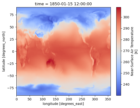
Select time#
Select a specific time
dset['tas'].sel(time=cftime.DatetimeNoLeap(1850, 1, 15, 12, 0, 0, 0, 2, 15)).plot(cmap = 'coolwarm')
<matplotlib.collections.QuadMesh at 0x7fd228d96dd0>
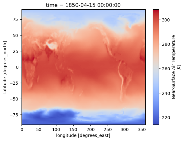
select the nearest time. Here from 1st April 1950
dset['tas'].sel(time=cftime.DatetimeNoLeap(1850, 4, 1), method='nearest').plot(cmap='coolwarm')
<matplotlib.collections.QuadMesh at 0x7fd220492c90>
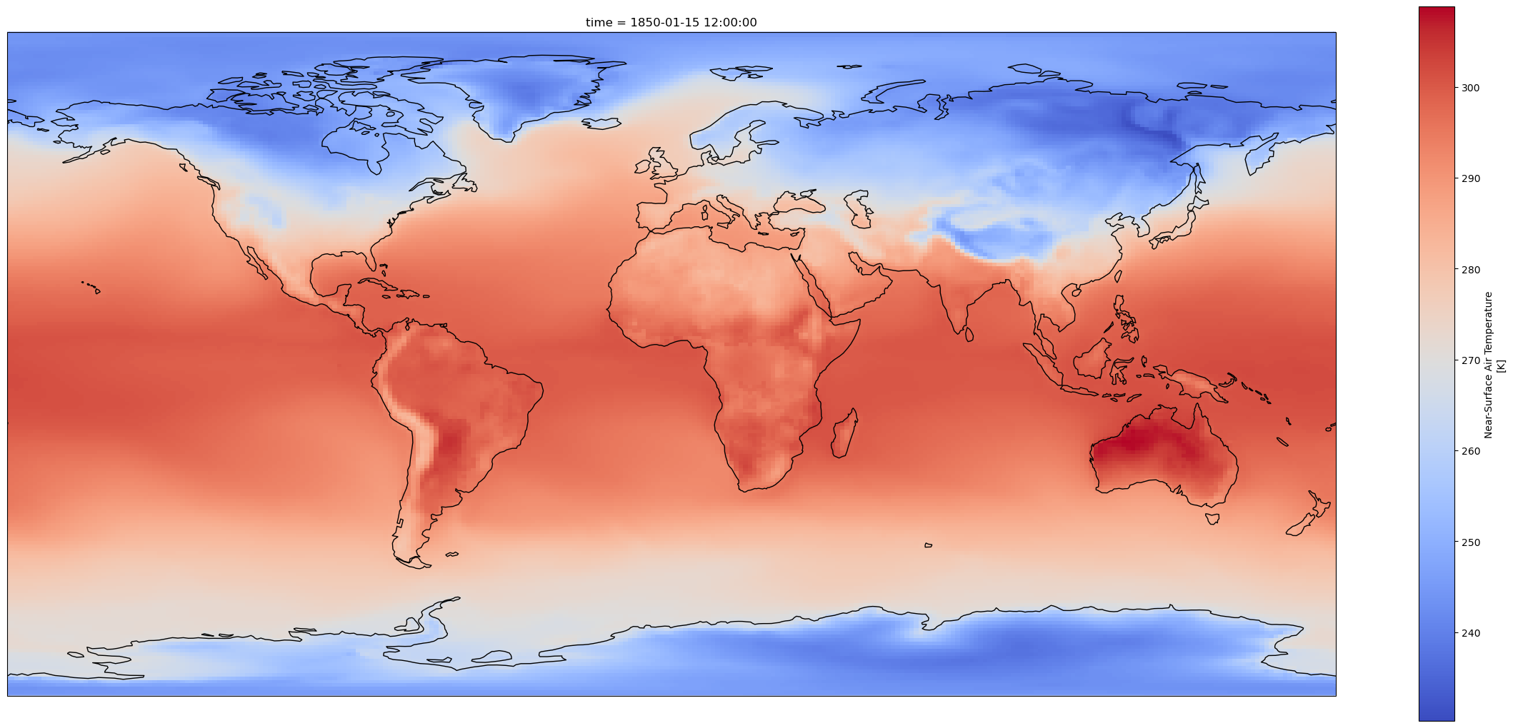
Customize plot#
Set the size of the figure and add coastlines#
fig = plt.figure(1, figsize=[30,13])

# Set the projection to use for plotting
ax = plt.subplot(1, 1, 1, projection=ccrs.PlateCarree())
ax.coastlines()

# Pass ax as an argument when plotting. Here we assume data is in the same coordinate reference system than the projection chosen for plotting
# isel allows to select by indices instead of the time values
dset['tas'].isel(time=0).plot.pcolormesh(ax=ax, cmap='coolwarm')
<cartopy.mpl.geocollection.GeoQuadMesh at 0x7fd228e4f610>
Change plotting projection#
fig = plt.figure(1, figsize=[10,10])
# We're using cartopy and are plotting in Orthographic projection
# (see documentation on cartopy)
ax = plt.subplot(1, 1, 1, projection=ccrs.Orthographic(0, 90))
ax.coastlines()
# We need to project our data to the new Orthographic projection and for this we use `transform`.
# we set the original data projection in transform (here PlateCarree)
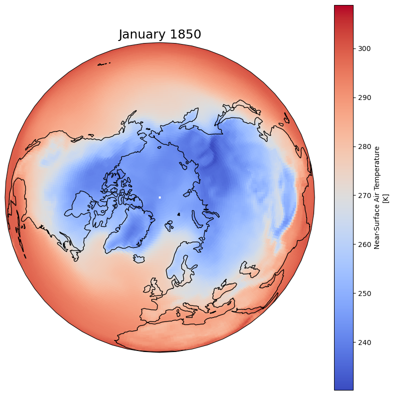
dset['tas'].isel(time=0).plot(ax=ax, transform=ccrs.PlateCarree(), cmap='coolwarm')
# One way to customize your title
plt.title(dset.time.values[0].strftime("%B %Y"), fontsize=18)
Text(0.5, 1.0, 'January 1850')
Choose the extent of values#
Fix your minimum and maximum values in your plot and
Use extend so values below the minimum and max
fig = plt.figure(1, figsize=[10,10])
ax = plt.subplot(1, 1, 1, projection=ccrs.Orthographic(0, 90))
ax.coastlines()
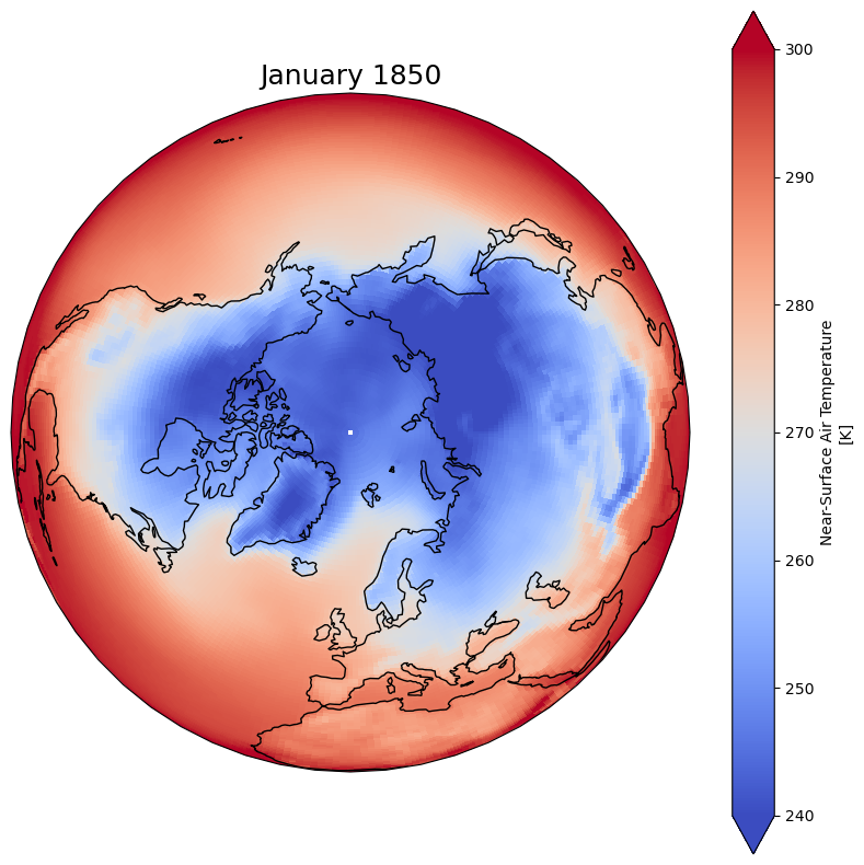
# Fix extent
minval = 240
maxval = 300
# pass extent with vmin and vmax parameters
dset['tas'].isel(time=0).plot(ax=ax, vmin=minval, vmax=maxval, transform=ccrs.PlateCarree(), cmap='coolwarm')
# One way to customize your title
plt.title(dset.time.values[0].strftime("%B %Y"), fontsize=18)
Text(0.5, 1.0, 'January 1850')
Multiplots#
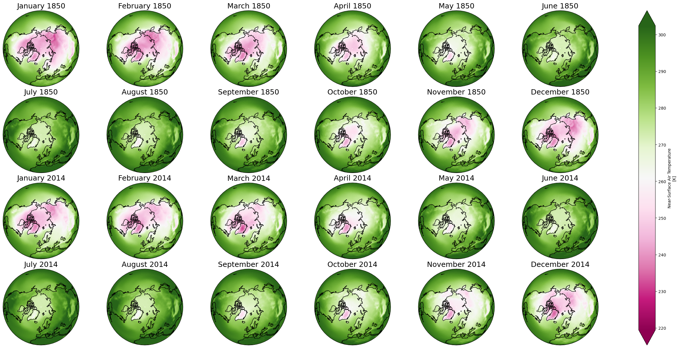
Faceting#
proj_plot = ccrs.Orthographic(0, 90)

p = dset['tas'].sel(time = dset.time.dt.year.isin([1850, 2014])).plot(x='lon', y='lat',
                                                                 transform=ccrs.PlateCarree(),
                                                                 aspect=dset.dims["lon"] / dset.dims["lat"],  # for a sensible figsize
                                                                 subplot_kws={"projection": proj_plot},
                                                                 col='time', col_wrap=6, robust=True, cmap='PiYG')
# We have to set the map's options on all four axes
for ax,i in zip(p.axes.flat,  dset.time.sel(time = dset.time.dt.year.isin([1850, 2014])).values):
    ax.coastlines()
    ax.set_title(i.strftime("%B %Y"), fontsize=18)
/tmp/ipykernel_1437/1975360723.py:9: DeprecationWarning: self.axes is deprecated since 2022.11 in order to align with matplotlibs plt.subplots, use self.axs instead.
  for ax,i in zip(p.axes.flat,  dset.time.sel(time = dset.time.dt.year.isin([1850, 2014])).values):
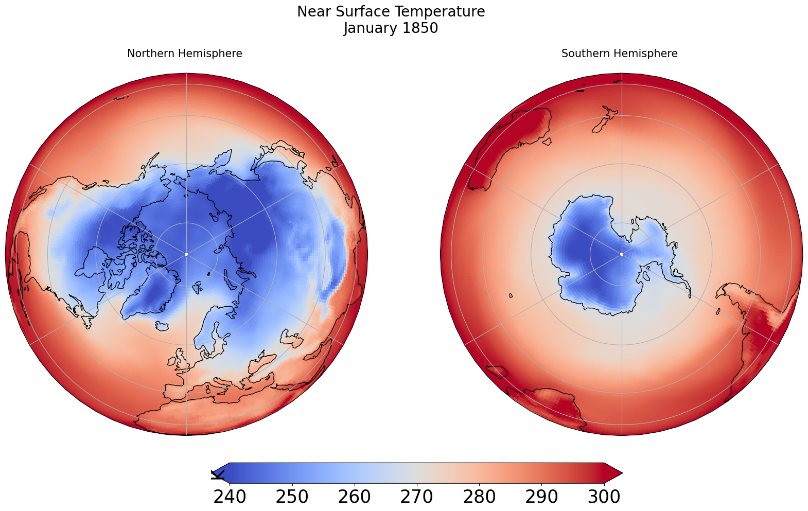
Combine plots with different projections#
fig = plt.figure(1, figsize=[20,10])

# Fix extent
minval = 240
maxval = 300

# Plot 1 for Northern Hemisphere subplot argument (nrows, ncols, nplot)
# here 1 row, 2 columns and 1st plot
ax1 = plt.subplot(1, 2, 1, projection=ccrs.Orthographic(0, 90))

# Plot 2 for Southern Hemisphere
# 2nd plot
ax2 = plt.subplot(1, 2, 2, projection=ccrs.Orthographic(180, -90))

tsel = 0
for ax,t in zip([ax1, ax2], ["Northern", "Southern"]):
    map = dset['tas'].isel(time=tsel).plot(ax=ax, vmin=minval, vmax=maxval,
                                           transform=ccrs.PlateCarree(),
                                           cmap='coolwarm',
                                           add_colorbar=False)
    ax.set_title(t + " Hemisphere \n" , fontsize=15)
    ax.coastlines()
    ax.gridlines()

# Title for both plots
fig.suptitle('Near Surface Temperature\n' + dset.time.values[tsel].strftime("%B %Y"), fontsize=20)


cb_ax = fig.add_axes([0.325, 0.05, 0.4, 0.04])

cbar = plt.colorbar(map, cax=cb_ax, extend='both', orientation='horizontal', fraction=0.046, pad=0.04)
cbar.ax.tick_params(labelsize=25)
cbar.ax.set_ylabel('K', fontsize=25)
Text(0, 0.5, 'K')