Plot ESM data on unstructured grids with psyplot

This notebook introduces you to the mapplot function of the package psyplot and its plugin psy_maps. It is suitable to plot maps from data on unstructured grids like the ones from ICON and FESOM.

We therefore search for the corresponding data in the CMIP6 data pool with intake-esm. Afterwards, we open a file with xarray and configure the opened xarray dataset as well as psyplot for a map plot.

This Jupyter notebook is meant to run in the Jupyterhub server of the German Climate Computing Center DKRZ. The DKRZ hosts the CMIP data pool including 4 petabytes of CMIP6 data. Please, choose the Python 3 unstable kernel on the Kernel tab above, it contains all the common geoscience packages. See more information on how to run Jupyter notebooks at DKRZ here.

Running this Jupyter notebook in your premise, which is also known as client-side computing, will require that you install the necessary packages intake, xarray, maplotlib, psyplot, psy_maps

and either download the data or use the opendap_url column of the intake catalog if available.

Learning Objectives

• How to access data on an unstructured grid from the DKRZ CMIP data pool with intake-esm

• How to subset data with xarray

• How to visualize the results with matplotlib, psyplot and psy_maps.

import psyplot.project as psy
import matplotlib as mpl
import xarray as xr
import intake

We open a swift catalog from dkrz cloud which is accessible without authentication.

# Path to master catalog on the DKRZ server
#dkrz_catalog=intake.open_catalog(["https://dkrz.de/s/intake"])
#
#only for the web page we need to take the original link:
parent_col=intake.open_catalog(["https://gitlab.dkrz.de/data-infrastructure-services/intake-esm/-/raw/master/esm-collections/cloud-access/dkrz_catalog.yaml"])
list(parent_col)

['dkrz_cmip5_archive',
 'dkrz_cmip5_disk',
 'dkrz_cmip6_cloud',
 'dkrz_cmip6_disk',
 'dkrz_cordex_disk',
 'dkrz_dyamond-winter_disk',
 'dkrz_era5_disk',
 'dkrz_monsoon_disk',
 'dkrz_mpige_disk',
 'dkrz_nextgems_disk',
 'dkrz_palmod2_disk']

col=parent_col["dkrz_cmip6_disk"]
col.df["uri"]=col.df["uri"].str.replace("lustre/","lustre02/") 

In this example, we aim at plotting the Sea Surface Temperature tos of the upper boundary of the liquid ocean, including temperatures below sea-ice and floating ice shelves from the earth system model AWI-CM-1-1-MR. We therefore search for tos in the catalog for monthly frequency. We only use one realization r1i1p1f1 of one experiment only.

tos=col.search(source_id="AWI-CM-1-1-MR",
               experiment_id="ssp370",
               variable_id="tos",
               table_id="Omon",
              member_id="r1i1p1f1")

tos.df["uri"].to_list()[0]

'/work/ik1017/CMIP6/data/CMIP6/ScenarioMIP/AWI/AWI-CM-1-1-MR/ssp370/r1i1p1f1/Omon/tos/gn/v20181218/tos_Omon_AWI-CM-1-1-MR_ssp370_r1i1p1f1_gn_201501-202012.nc'

We now open the file on the mistral lustre file system. Note that if you work remotely, you could try to use opendap_url instead of path.

dset = xr.open_dataset(tos.df["uri"].to_list()[0],
                      decode_cf=True,
                      chunks={"time":1},
                      lock=False)
dset

<xarray.Dataset>
Dimensions:    (time: 72, bnds: 2, ncells: 830305, vertices: 16)
Coordinates:
  * time       (time) datetime64[ns] 2015-01-16T12:00:00 ... 2020-12-16T12:00:00
    lat        (ncells) float64 dask.array<chunksize=(830305,), meta=np.ndarray>
    lon        (ncells) float64 dask.array<chunksize=(830305,), meta=np.ndarray>
Dimensions without coordinates: bnds, ncells, vertices
Data variables:
    time_bnds  (time, bnds) datetime64[ns] dask.array<chunksize=(1, 2), meta=np.ndarray>
    tos        (time, ncells) float32 dask.array<chunksize=(1, 830305), meta=np.ndarray>
    lat_bnds   (ncells, vertices) float64 dask.array<chunksize=(830305, 16), meta=np.ndarray>
    lon_bnds   (ncells, vertices) float64 dask.array<chunksize=(830305, 16), meta=np.ndarray>
Attributes: (12/39)
    frequency:              mon
    Conventions:            CF-1.7 CMIP-6.2
    creation_date:          2018-12-18T12:00:00Z
    data_specs_version:     01.00.27
    experiment:             ssp370
    experiment_id:          ssp370
    ...                     ...
    parent_experiment_id:   historical
    parent_mip_era:         CMIP6
    parent_source_id:       AWI-CM-1-1-MR
    parent_time_units:      days since 1850-1-1
    parent_variant_label:   r1i1p1f1
    activity_id:            ScenarioMIP AerChemMIP

xarray.Dataset

• Dimensions:
  • time: 72
  • bnds: 2
  • ncells: 830305
  • vertices: 16
• Coordinates: (3)
  • time
    (time)
    datetime64[ns]
    2015-01-16T12:00:00 ... 2020-12-...

    standard_name :

    time

    long_name :

    time

    bounds :

    time_bnds

    axis :

    T

    array(['2015-01-16T12:00:00.000000000', '2015-02-15T00:00:00.000000000',
           '2015-03-16T12:00:00.000000000', '2015-04-16T00:00:00.000000000',
           '2015-05-16T12:00:00.000000000', '2015-06-16T00:00:00.000000000',
           '2015-07-16T12:00:00.000000000', '2015-08-16T12:00:00.000000000',
           '2015-09-16T00:00:00.000000000', '2015-10-16T12:00:00.000000000',
           '2015-11-16T00:00:00.000000000', '2015-12-16T12:00:00.000000000',
           '2016-01-16T12:00:00.000000000', '2016-02-15T12:00:00.000000000',
           '2016-03-16T12:00:00.000000000', '2016-04-16T00:00:00.000000000',
           '2016-05-16T12:00:00.000000000', '2016-06-16T00:00:00.000000000',
           '2016-07-16T12:00:00.000000000', '2016-08-16T12:00:00.000000000',
           '2016-09-16T00:00:00.000000000', '2016-10-16T12:00:00.000000000',
           '2016-11-16T00:00:00.000000000', '2016-12-16T12:00:00.000000000',
           '2017-01-16T12:00:00.000000000', '2017-02-15T00:00:00.000000000',
           '2017-03-16T12:00:00.000000000', '2017-04-16T00:00:00.000000000',
           '2017-05-16T12:00:00.000000000', '2017-06-16T00:00:00.000000000',
           '2017-07-16T12:00:00.000000000', '2017-08-16T12:00:00.000000000',
           '2017-09-16T00:00:00.000000000', '2017-10-16T12:00:00.000000000',
           '2017-11-16T00:00:00.000000000', '2017-12-16T12:00:00.000000000',
           '2018-01-16T12:00:00.000000000', '2018-02-15T00:00:00.000000000',
           '2018-03-16T12:00:00.000000000', '2018-04-16T00:00:00.000000000',
           '2018-05-16T12:00:00.000000000', '2018-06-16T00:00:00.000000000',
           '2018-07-16T12:00:00.000000000', '2018-08-16T12:00:00.000000000',
           '2018-09-16T00:00:00.000000000', '2018-10-16T12:00:00.000000000',
           '2018-11-16T00:00:00.000000000', '2018-12-16T12:00:00.000000000',
           '2019-01-16T12:00:00.000000000', '2019-02-15T00:00:00.000000000',
           '2019-03-16T12:00:00.000000000', '2019-04-16T00:00:00.000000000',
           '2019-05-16T12:00:00.000000000', '2019-06-16T00:00:00.000000000',
           '2019-07-16T12:00:00.000000000', '2019-08-16T12:00:00.000000000',
           '2019-09-16T00:00:00.000000000', '2019-10-16T12:00:00.000000000',
           '2019-11-16T00:00:00.000000000', '2019-12-16T12:00:00.000000000',
           '2020-01-16T12:00:00.000000000', '2020-02-15T12:00:00.000000000',
           '2020-03-16T12:00:00.000000000', '2020-04-16T00:00:00.000000000',
           '2020-05-16T12:00:00.000000000', '2020-06-16T00:00:00.000000000',
           '2020-07-16T12:00:00.000000000', '2020-08-16T12:00:00.000000000',
           '2020-09-16T00:00:00.000000000', '2020-10-16T12:00:00.000000000',
           '2020-11-16T00:00:00.000000000', '2020-12-16T12:00:00.000000000'],
          dtype='datetime64[ns]')

  • lat
    (ncells)
    float64
    dask.array<chunksize=(830305,), meta=np.ndarray>

    units :

    degrees_north

    standard_name :

    latitude

    bounds :

    lat_bnds

    Array Chunk Bytes 6.33 MiB 6.33 MiB Shape (830305,) (830305,) Dask graph 1 chunks in 2 graph layers Data type float64 numpy.ndarray

  • lon
    (ncells)
    float64
    dask.array<chunksize=(830305,), meta=np.ndarray>

    units :

    degrees_east

    standard_name :

    longitude

    bounds :

    lon_bnds

    Array Chunk Bytes 6.33 MiB 6.33 MiB Shape (830305,) (830305,) Dask graph 1 chunks in 2 graph layers Data type float64 numpy.ndarray

• Data variables: (4)
  • time_bnds
    (time, bnds)
    datetime64[ns]
    dask.array<chunksize=(1, 2), meta=np.ndarray>

    Array Chunk Bytes 1.12 kiB 16 B Shape (72, 2) (1, 2) Dask graph 72 chunks in 2 graph layers Data type datetime64[ns] numpy.ndarray

  • tos
    (time, ncells)
    float32
    dask.array<chunksize=(1, 830305), meta=np.ndarray>

    units :

    degC

    CDI_grid_type :

    unstructured

    description :

    Temperature of upper boundary of the liquid ocean, including temperatures below sea-ice and floating ice shelves.

    standard_name :

    sea_surface_temperature

    cell_methods :

    area: mean where sea time: mean

    cell_measures :

    area: areacello

    Array Chunk Bytes 228.05 MiB 3.17 MiB Shape (72, 830305) (1, 830305) Dask graph 72 chunks in 2 graph layers Data type float32 numpy.ndarray

  • lat_bnds
    (ncells, vertices)
    float64
    dask.array<chunksize=(830305, 16), meta=np.ndarray>

    Array Chunk Bytes 101.36 MiB 101.36 MiB Shape (830305, 16) (830305, 16) Dask graph 1 chunks in 2 graph layers Data type float64 numpy.ndarray

  • lon_bnds
    (ncells, vertices)
    float64
    dask.array<chunksize=(830305, 16), meta=np.ndarray>

    Array Chunk Bytes 101.36 MiB 101.36 MiB Shape (830305, 16) (830305, 16) Dask graph 1 chunks in 2 graph layers Data type float64 numpy.ndarray

• Indexes: (1)
  • time
    PandasIndex

    PandasIndex(DatetimeIndex(['2015-01-16 12:00:00', '2015-02-15 00:00:00',
                   '2015-03-16 12:00:00', '2015-04-16 00:00:00',
                   '2015-05-16 12:00:00', '2015-06-16 00:00:00',
                   '2015-07-16 12:00:00', '2015-08-16 12:00:00',
                   '2015-09-16 00:00:00', '2015-10-16 12:00:00',
                   '2015-11-16 00:00:00', '2015-12-16 12:00:00',
                   '2016-01-16 12:00:00', '2016-02-15 12:00:00',
                   '2016-03-16 12:00:00', '2016-04-16 00:00:00',
                   '2016-05-16 12:00:00', '2016-06-16 00:00:00',
                   '2016-07-16 12:00:00', '2016-08-16 12:00:00',
                   '2016-09-16 00:00:00', '2016-10-16 12:00:00',
                   '2016-11-16 00:00:00', '2016-12-16 12:00:00',
                   '2017-01-16 12:00:00', '2017-02-15 00:00:00',
                   '2017-03-16 12:00:00', '2017-04-16 00:00:00',
                   '2017-05-16 12:00:00', '2017-06-16 00:00:00',
                   '2017-07-16 12:00:00', '2017-08-16 12:00:00',
                   '2017-09-16 00:00:00', '2017-10-16 12:00:00',
                   '2017-11-16 00:00:00', '2017-12-16 12:00:00',
                   '2018-01-16 12:00:00', '2018-02-15 00:00:00',
                   '2018-03-16 12:00:00', '2018-04-16 00:00:00',
                   '2018-05-16 12:00:00', '2018-06-16 00:00:00',
                   '2018-07-16 12:00:00', '2018-08-16 12:00:00',
                   '2018-09-16 00:00:00', '2018-10-16 12:00:00',
                   '2018-11-16 00:00:00', '2018-12-16 12:00:00',
                   '2019-01-16 12:00:00', '2019-02-15 00:00:00',
                   '2019-03-16 12:00:00', '2019-04-16 00:00:00',
                   '2019-05-16 12:00:00', '2019-06-16 00:00:00',
                   '2019-07-16 12:00:00', '2019-08-16 12:00:00',
                   '2019-09-16 00:00:00', '2019-10-16 12:00:00',
                   '2019-11-16 00:00:00', '2019-12-16 12:00:00',
                   '2020-01-16 12:00:00', '2020-02-15 12:00:00',
                   '2020-03-16 12:00:00', '2020-04-16 00:00:00',
                   '2020-05-16 12:00:00', '2020-06-16 00:00:00',
                   '2020-07-16 12:00:00', '2020-08-16 12:00:00',
                   '2020-09-16 00:00:00', '2020-10-16 12:00:00',
                   '2020-11-16 00:00:00', '2020-12-16 12:00:00'],
                  dtype='datetime64[ns]', name='time', freq=None))

• Attributes: (39)

  frequency :

  mon

  Conventions :

  CF-1.7 CMIP-6.2

  creation_date :

  2018-12-18T12:00:00Z

  data_specs_version :

  01.00.27

  experiment :

  ssp370

  experiment_id :

  ssp370

  forcing_index :

  1

  further_info_url :

  https://furtherinfo.es-doc.org/CMIP6.AWI.AWI-CM-1-1-MR.ssp370.none.r1i1p1f1

  grid :

  FESOM 1.4 (unstructured grid in the horizontal with 830305 wet nodes; 46 levels; top grid cell 0-5 m)

  grid_label :

  gn

  initialization_index :

  1

  institution :

  Alfred Wegener Institute, Helmholtz Centre for Polar and Marine Research, Am Handelshafen 12, 27570 Bremerhaven, Germany

  institution_id :

  AWI

  license :

  CMIP6 model data produced by Alfred Wegener Institute, Helmholtz Centre for Polar and Marine Research, Am Handelshafen 12, 27570 Bremerhaven, Germany is licensed under a Creative Commons Attribution-ShareAlike 4.0 International License (https://creativecommons.org/licenses/). Consult https://pcmdi.llnl.gov/CMIP6/TermsOfUse for terms of use governing CMIP6 output, including citation requirements and proper acknowledgment. Further information about this data, including some limitations, can be found via the further_info_url (recorded as a global attribute in this file). The data producers and data providers make no warranty, either express or implied, including, but not limited to, warranties of merchantability and fitness for a particular purpose. All liabilities arising from the supply of the information (including any liability arising in negligence) are excluded to the fullest extent permitted by law.

  mip_era :

  CMIP6

  nominal_resolution :

  25 km

  physics_index :

  1

  product :

  model-output

  realization_index :

  1

  realm :

  ocean

  source :

  AWI-CM-1-1-MR

  source_id :

  AWI-CM-1-1-MR

  source_type :

  AOGCM

  sub_experiment :

  none

  sub_experiment_id :

  none

  table_id :

  Omon

  tracking_id :

  hdl:21.14100/9ac88215-8062-416c-b0d3-a4f7e14cadb1

  variable_id :

  tos

  variant_label :

  r1i1p1f1

  branch_method :

  standard

  branch_time_in_child :

  0.0

  branch_time_in_parent :

  60265.0

  parent_activity_id :

  CMIP

  parent_experiment_id :

  historical

  parent_mip_era :

  CMIP6

  parent_source_id :

  AWI-CM-1-1-MR

  parent_time_units :

  days since 1850-1-1

  parent_variant_label :

  r1i1p1f1

  activity_id :

  ScenarioMIP AerChemMIP

In order to make tos plottable, we set the following configuration.

• The CDI_grid_type is a keyword for psyplot. It must match the grid type of the source model.

• Coordinates are not fully recognized by xarray so that we have to add some manually (version from Dec 2020).

dset["tos"]["CDI_grid_type"]="unstructured"
coordlist=["vertices_latitude", "vertices_longitude", "lat_bnds", "lon_bnds"]
dset=dset.set_coords([coord for coord in dset.data_vars if coord in coordlist])

The following is based on the psyplot example. We set a resoltion for the land sea mask lsm and a color map via cmap.

psy.rcParams['plotter.maps.xgrid'] = False
psy.rcParams['plotter.maps.ygrid'] = False
mpl.rcParams['figure.figsize'] = [10, 8.]

def plot_unstructured():
    iconplot11=psy.plot.mapplot(
        dset, name="tos", cmap='rainbow',
        clabel=dset["tos"].description,
        stock_img=True, lsm='50m')

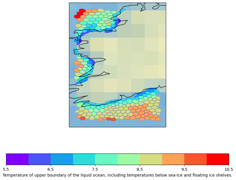
We now do the same with a smaller subset to highlight the fine resolution and the structure of the AWI ocean model FESOM. We first subset the data because otherwise plotting takes too long. We choose indices of dimensions with the xarray function isel. We select a slice of two time steps and focus on a region Ireland. We have to save the data to an intermediate file test.nc because otherwise we receive an error.

dset["lat"]=dset.lat.load()
dset["lon"]=dset.lon.load()
dset2 = dset.isel(time=slice(1,2)).where( (dset.lon > -10. ) &
                    (dset.lon < 50. ) &
                    (dset.lat > 40. ) &
                    (dset.lat < 70. ), drop=True).drop("time_bnds")

dset2

<xarray.Dataset>
Dimensions:   (time: 1, ncells: 28844, vertices: 16)
Coordinates:
  * time      (time) datetime64[ns] 2015-02-15
    lat       (ncells) float64 69.74 69.16 69.17 69.72 ... 69.8 67.23 42.17
    lat_bnds  (ncells, vertices) float64 dask.array<chunksize=(28844, 16), meta=np.ndarray>
    lon       (ncells) float64 -8.645 -9.653 -5.883 -6.825 ... 47.55 47.76 18.49
    lon_bnds  (ncells, vertices) float64 dask.array<chunksize=(28844, 16), meta=np.ndarray>
Dimensions without coordinates: ncells, vertices
Data variables:
    tos       (time, ncells) float32 dask.array<chunksize=(1, 28844), meta=np.ndarray>
Attributes: (12/39)
    frequency:              mon
    Conventions:            CF-1.7 CMIP-6.2
    creation_date:          2018-12-18T12:00:00Z
    data_specs_version:     01.00.27
    experiment:             ssp370
    experiment_id:          ssp370
    ...                     ...
    parent_experiment_id:   historical
    parent_mip_era:         CMIP6
    parent_source_id:       AWI-CM-1-1-MR
    parent_time_units:      days since 1850-1-1
    parent_variant_label:   r1i1p1f1
    activity_id:            ScenarioMIP AerChemMIP

xarray.Dataset

• Dimensions:
  • time: 1
  • ncells: 28844
  • vertices: 16
• Coordinates: (5)
  • time
    (time)
    datetime64[ns]
    2015-02-15

    standard_name :

    time

    long_name :

    time

    bounds :

    time_bnds

    axis :

    T

    array(['2015-02-15T00:00:00.000000000'], dtype='datetime64[ns]')

  • lat
    (ncells)
    float64
    69.74 69.16 69.17 ... 67.23 42.17

    units :

    degrees_north

    standard_name :

    latitude

    bounds :

    lat_bnds

    array([69.7446878 , 69.16446039, 69.17367568, ..., 69.79736089,
           67.23437368, 42.16660379])

  • lat_bnds
    (ncells, vertices)
    float64
    dask.array<chunksize=(28844, 16), meta=np.ndarray>

    Array Chunk Bytes 3.52 MiB 3.52 MiB Shape (28844, 16) (28844, 16) Dask graph 1 chunks in 3 graph layers Data type float64 numpy.ndarray

  • lon
    (ncells)
    float64
    -8.645 -9.653 ... 47.76 18.49

    units :

    degrees_east

    standard_name :

    longitude

    bounds :

    lon_bnds

    array([-8.6446149 , -9.65269778, -5.88277498, ..., 47.55482987,
           47.7602283 , 18.49120667])

  • lon_bnds
    (ncells, vertices)
    float64
    dask.array<chunksize=(28844, 16), meta=np.ndarray>

    Array Chunk Bytes 3.52 MiB 3.52 MiB Shape (28844, 16) (28844, 16) Dask graph 1 chunks in 3 graph layers Data type float64 numpy.ndarray

• Data variables: (1)
  • tos
    (time, ncells)
    float32
    dask.array<chunksize=(1, 28844), meta=np.ndarray>

    units :

    degC

    CDI_grid_type :

    unstructured

    description :

    Temperature of upper boundary of the liquid ocean, including temperatures below sea-ice and floating ice shelves.

    standard_name :

    sea_surface_temperature

    cell_methods :

    area: mean where sea time: mean

    cell_measures :

    area: areacello

    Array Chunk Bytes 112.67 kiB 112.67 kiB Shape (1, 28844) (1, 28844) Dask graph 1 chunks in 6 graph layers Data type float32 numpy.ndarray

• Indexes: (1)
  • time
    PandasIndex

    PandasIndex(DatetimeIndex(['2015-02-15'], dtype='datetime64[ns]', name='time', freq=None))

• Attributes: (39)

  frequency :

  mon

  Conventions :

  CF-1.7 CMIP-6.2

  creation_date :

  2018-12-18T12:00:00Z

  data_specs_version :

  01.00.27

  experiment :

  ssp370

  experiment_id :

  ssp370

  forcing_index :

  1

  further_info_url :

  https://furtherinfo.es-doc.org/CMIP6.AWI.AWI-CM-1-1-MR.ssp370.none.r1i1p1f1

  grid :

  FESOM 1.4 (unstructured grid in the horizontal with 830305 wet nodes; 46 levels; top grid cell 0-5 m)

  grid_label :

  gn

  initialization_index :

  1

  institution :

  Alfred Wegener Institute, Helmholtz Centre for Polar and Marine Research, Am Handelshafen 12, 27570 Bremerhaven, Germany

  institution_id :

  AWI

  license :

  CMIP6 model data produced by Alfred Wegener Institute, Helmholtz Centre for Polar and Marine Research, Am Handelshafen 12, 27570 Bremerhaven, Germany is licensed under a Creative Commons Attribution-ShareAlike 4.0 International License (https://creativecommons.org/licenses/). Consult https://pcmdi.llnl.gov/CMIP6/TermsOfUse for terms of use governing CMIP6 output, including citation requirements and proper acknowledgment. Further information about this data, including some limitations, can be found via the further_info_url (recorded as a global attribute in this file). The data producers and data providers make no warranty, either express or implied, including, but not limited to, warranties of merchantability and fitness for a particular purpose. All liabilities arising from the supply of the information (including any liability arising in negligence) are excluded to the fullest extent permitted by law.

  mip_era :

  CMIP6

  nominal_resolution :

  25 km

  physics_index :

  1

  product :

  model-output

  realization_index :

  1

  realm :

  ocean

  source :

  AWI-CM-1-1-MR

  source_id :

  AWI-CM-1-1-MR

  source_type :

  AOGCM

  sub_experiment :

  none

  sub_experiment_id :

  none

  table_id :

  Omon

  tracking_id :

  hdl:21.14100/9ac88215-8062-416c-b0d3-a4f7e14cadb1

  variable_id :

  tos

  variant_label :

  r1i1p1f1

  branch_method :

  standard

  branch_time_in_child :

  0.0

  branch_time_in_parent :

  60265.0

  parent_activity_id :

  CMIP

  parent_experiment_id :

  historical

  parent_mip_era :

  CMIP6

  parent_source_id :

  AWI-CM-1-1-MR

  parent_time_units :

  days since 1850-1-1

  parent_variant_label :

  r1i1p1f1

  activity_id :

  ScenarioMIP AerChemMIP

dset2.to_netcdf("test.nc")

dset2.close()

dset=xr.open_dataset("test.nc",
                      decode_cf=True)

dset["tos"]["CDI_grid_type"]="unstructured"
coordlist=["vertices_latitude", "vertices_longitude", "lat_bnds", "lon_bnds"]
dset=dset.set_coords([coord for coord in dset.data_vars if coord in coordlist])

psy.plot.mapplot(
    dset, name="tos", cmap='rainbow',
    lonlatbox='Ireland',
    clabel=dset["tos"].description,
    stock_img=True,
    lsm='50m',
    datagrid=dict(c='b', lw=0.2)).show()

/envs/lib/python3.11/site-packages/cartopy/io/__init__.py:241: DownloadWarning: Downloading: https://naturalearth.s3.amazonaws.com/50m_physical/ne_50m_coastline.zip
  warnings.warn(f'Downloading: {url}', DownloadWarning)

dset.close()

Used data

• Semmler et al., 2019: AWI AWI-CM1.1MR model output prepared for CMIP6

We acknowledge the CMIP community for providing the climate model data, retained and globally distributed in the framework of the ESGF. The CMIP data of this study were replicated and made available for this study by the DKRZ.”